The average said it was fine.
I built a weekly demand forecast that beat every standard method I tried, with almost no bias overall. I was ready to call it done. Then I split one number a different way.
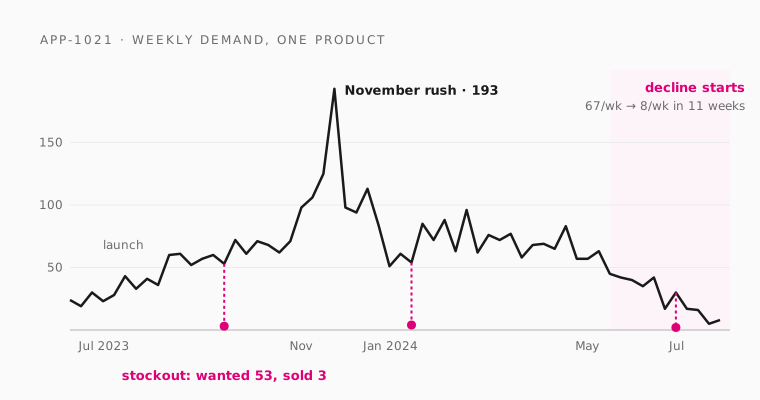
In May 2024, a clothing item in an online shop, product APP-1021, was selling about 67 a week. It had been for months. It had launched the summer before, ramped up, and sailed through a November rush of 193 in a single week.
Eleven weeks later, it was selling 8 a week, and then it was gone.
Look at its history the week before it started falling and nothing hints at what's coming. Anything that reads that history, a person or a model, says the same thing: keep ordering about 65 a week. Over those eleven weeks, that's roughly 740 units, against about 300 that customers actually wanted.
I spent most of this project not noticing products like APP-1021. The forecast I built looked excellent, and the number I was using to judge it said so.
The job: how much should be on the shelf?
An online shop has one question it asks every week: how many of each product should be in the warehouse four weeks from now, and three months from now? Order too few and customers leave empty-handed. Order too many and cash sits on a shelf until it gets marked down.
I built a forecast to answer that for 320 products, using a public Kaggle dataset of weekly sales from July 2022 to December 2024. The data is synthetic. That's a limitation, but it's also why I picked it: it records the true demand behind every week, including weeks the shelf was empty. Real sales data never shows you that, so here every forecast can be scored against what customers actually wanted.
The forecast looked finished
I tested it the honest way. I trained only on weeks up to a cutoff date, forecast the weeks after it, and repeated that across 2024, including the November peak. Then I compared it with the methods a planner would normally use:
| Method | Units missed, 4 weeks ahead | Units missed, 3 months ahead |
|---|---|---|
| My forecast | 15.2% | 18.9% |
| Best standard method at each range | 20.5% | 23.8% |
| Same week last year | 28.5% | 27.9% |
That's a quarter less error than the best alternative at four weeks. Its overall bias, whether it leans too high or too low, was −1.3%: a hair under, which is about as close to neutral as a forecast gets.
I was writing it up as done. Then I split that −1.3% by where each product was in its life.
Then I split the average
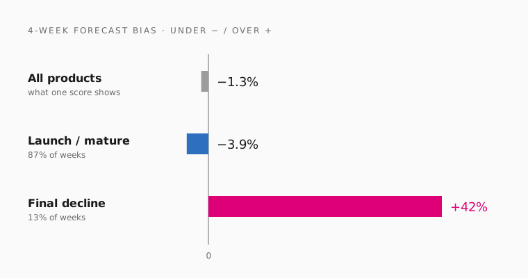 One number for all products, then the same number split by product stage.
| Product stage | Share of forecast weeks | Lean, 4 weeks | Lean, 3 months |
|---|---|---|---|
| Launch or mature | 87% | −3.9% | −7.2% |
| Final decline | 13% | +42% | +72% |
| All products | 100% | −1.3% | −3.2% |
Products like APP-1021 were only 13% of the weeks, so the 87% of healthy weeks outvoted them. The average wasn't wrong. It was answering a question nobody running a warehouse would ask.
Those two errors don't cost the same, either. Under-forecasting a healthy product loses a few sales. Over-forecasting a dying one fills the warehouse with something nobody will buy again, ordered three months ahead at the worst possible time.
The cause is the APP-1021 problem. A product about to start its final decline looks, in its history, exactly like a healthy one. My forecast does track recent trend, but that only catches the slide once it has started, and by then the 3-month order is placed.
The rest of the forecast held up. Here's how it was built, and why each step is there.
How the forecast is built
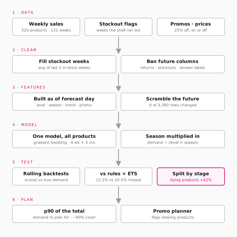 Six stages. Each one exists because a forecast can quietly go wrong there.
Sales history isn't the same as demand
Go back to APP-1021. In the week of 1 July 2024, it sold 2 units. Customers wanted 30. The shelf was empty.
A sales record tells you what was sold, not what people wanted. Those are the same number until a product runs out. Across this dataset, a stockout week captured just 14% of real demand. Leave those weeks in, and the forecast sees demand collapse for no reason, learns to aim low, and leaves the shelf too empty next time.
A shop always knows which weeks it was out of stock, so the fix is simple. I replaced each stockout week with the product's average from its last two in-stock weeks. Only earlier weeks are used, so the fill never borrows from the future. To see what that was worth, I trained the same forecast three ways:
| Trained on | Units missed |
|---|---|
| Raw sales, stockout weeks left in | 17.6% |
| Stockout weeks filled | 15.2% |
| True demand (impossible in real life) | 14.9% |
One plain rule closed almost the whole gap to perfect data. No algorithm upgrade would have done that.
How do you stop a forecast from seeing the future?
A forecast made on 30 September can only use what was known on 30 September. Using anything else is called data leakage, and it's the fastest way to build a forecast that looks brilliant in testing and fails in real life. It's the same trap that inflated my ticket classifier by 33 points.
This dataset makes it easy to fall into. It has columns that are only known after the week is over, like returns, and two that are the simulator's own answer key, one of which marks exactly when a product starts dying. I banned all of them before building anything.
The forecast reads recent sales, the trend, the usual seasonal pattern for the week ahead, the same week last year, how long the product has been on sale, its price, and whether a promotion is planned, each worked out as of the forecast date. To prove nothing leaked, I scrambled every week after the forecast date and rebuilt everything. All 3,380 rows I tested came out identical.
One model learns from every product
The standard approach, a method called exponential smoothing (ETS), forecasts each product from its own history. To learn a yearly pattern like the November rush, it needs to see at least two of them. Not one product here had two years of history. APP-1021 saw a single November.
So I trained one model across all 320 products instead. It learns what November does from every product that has lived through one, then applies that to each product's own recent sales. The model is gradient boosting, which builds hundreds of small decision trees that each correct the last one's mistakes. I picked it because it handles a mix of numbers and categories with little preparation, and it can produce a cautious upper estimate as well as a central one.
One choice mattered more than the rest. Asked to predict sales directly, the model flattened seasonal peaks. From a 30 September forecast, it expected November to rise 1.22 times when the real rise was 1.49 times. So I gave it the seasonal pattern up front and asked it to predict only the difference from that. The peak came back to 1.40 times, and the model could spend its effort on promotions, trends and product age.
Order for a bad week, not an average one
A forecast is a middle guess, so real demand lands above it about half the time. Nobody stocks to a coin flip. A second model predicts a cautious upper figure, the p90: a level demand should stay under 9 times out of 10.
The trap is adding those weekly figures up for an order. Over four or thirteen weeks, a busy week and a quiet one partly cancel, so the sum overshoots. It covered 96–97% of real totals instead of 90%, which is stock bought for no reason. The planner instead shows the p90 of the total, scaled from how totals actually missed in testing. It covered about 90%, and it plans 2–8% less stock.
What it can't do yet
What this taught me
The forecast was finished long before I understood it. Everything I'd normally check said it was good, and it was good, for 87% of the weeks. The other 13% were where the money went.
So I'm curious: when you judge a forecast, or any model, what do you check besides the average?
Frequently asked questions
Why did the overall bias look fine when dying products were 42% off?
Dying products were only 13% of forecast weeks, and the other 87% were under-forecast by 3.9%. A small under-forecast on many weeks and a large over-forecast on a few cancel out to −1.3%. Splitting by product stage shows both errors.
What is a stockout week, and why fill it in?
It's a week the product ran out, so recorded sales show only what was on the shelf: 14% of real demand in this data. Left in, those weeks teach the forecast that demand collapsed. Filling each one with the average of the product's last two in-stock weeks cut error from 17.6% to 15.2%, close to the 14.9% possible with perfect data.
Why not use exponential smoothing (ETS), the standard method?
Per-product ETS needs two full years of history to learn a yearly pattern, and every product here had less. The textbook version missed 22.0% of units at 4 weeks and 33.7% at 3 months. One model trained across all products learns the season from all of them at once, and it missed 15.2% and 18.9%.
What does p90 mean?
It's a level demand should stay under 90% of the time. The planner shows the p90 of total demand over the period, which covered about 90% of real totals in testing. Adding up weekly p90s instead covered 96–97%, which means buying stock you didn't need.
How do you know the forecast doesn't use future information?
Every column was classified before modelling, and future-only columns were banned. Then I scrambled every week after each forecast date and rebuilt the inputs: all 3,380 rows tested were unchanged.
Is the data real?
No. It's a public Kaggle dataset of 320 synthetic products, which is what makes true demand available for scoring. The method carries over, but the numbers need revalidating on real sales.
Which tools did I use?
Python, pandas, scikit-learn's HistGradientBoosting for the forecast and the p90, statsforecast for the ETS baselines, and Shiny for Python for the promo planner.